In the era of big data, Excel stands out as a crucial spreadsheet software. It was one of the first to gain widespread popularity for efficiently handling data while maintaining user familiarity. Despite the years passing, Excel hasn’t lost relevance in the data world. In any industry, if you have to deal with data, you’ll most likely have to use Excel at some point.
With this Excel formulas cheat sheet, I aim to help you save time looking for formulas and focus on what really matters: managing and analyzing data. This way, you can make informed decisions based on a neatly manipulated spreadsheet.
Here, you will find the most common and useful formulas for different purposes with examples and short explanations, so you know when to use each.
Let’s head right into it.
These are some formulas that any user will constantly use in their Excel spreadsheets. Most likely, you will use at least one of these in any spreadsheet you create. Some of these basic Excel formulas are:
It adds the values in the range of cells you specify.
Examples and variations:
=SUM(B1;B5)
=SUM(B1:B5)
=SUM(B1;B5;12)
=SUM(B1:B3;B5;8)
It gives the average of the specific cells or range of cells you select.
Examples and variations:
=AVERAGE(C1:C5)
=AVERAGE(C1;C3;C4)
These identify the highest or lowest value in a range of cells
Examples and variations:
=MAX(B1:B5)
=MIN(B1:C5)
It counts how many of the cells in the range selected have a numeric value.
Examples and variations:
=COUNT(B1:B5)
=COUNT(C1:D4)
It raises a value to a certain power.
Examples and variations:
=POWER(C1;3)
=POWER(8;2)
=POWER(B3;4)
Round up numbers up or down to the nearest multiple, respectively.
Examples and variations:
=CEILING(B1;5)
=FLOOR(C1;5)
These formulas are used for working with text data, also known as strings. This can be used to make information more readable, allowing a more user-friendly presentation. Some of the most frequently used text manipulation formulas are:
It merges the content of two or more cells into one single cell. You can also add information between strings if needed.
Examples and variations:
=CONCATENATE(D2;" ";E2)
They return a determined portion of characters from a cell. LEFT returns the first characters, RIGHT returns the ones at the end, And MID returns the ones in the middle. You determine how many characters you’d like to be returned.
Examples and variations:
=LEFT(D1;5)
=RIGHT(D1;6)
=MID(D1;7;5)
It identifies double spaces and gets rid of them.
Examples and variations:
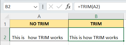
The extra spaces at the beginning and between “is” and “how” disappear.
It returns the number of characters present in a string.
Examples and variations:
=LEN(B1)
=LEN(D5)
These convert the text to uppercase or lowercase, respectively.
Examples and variations:
=UPPER(D4)
=LOWER(D3)
It capitalizes the first letter of each word in a string.
Examples and variations:

It converts numeric values into text but maintains a certain numeric format.
Examples and variations:
=CONCAT(K1;" - ";H1)
=CONCAT(K1;" - ";TEXT(H1;"mm/dd/yyyy"))
These formulas help with operations such as adding a certain number of days to a date or calculating end dates, taxation dates, and such. Some of the most common are:
Now returns the current system time and date, whereas TODAY gives just the current date.
Examples and variations:
If it’s 14:32 on July 17, 2006.
=NOW() Returns 17/07/2006 14:32,
=TODAY() Returns 17/07/2006
It turns the values you give into a date.
Examples and variations:
=DATE(2024;3;7)Returns 7/03/2024
Each returns the year, month, and day of a date.
=YEAR(A1)Returns 2024
=MONTH(A1)Returns 4
=DAY(A1)Returns 1
It calculates the date after a specified number of months before or after a given date.
Examples and variations:
=EDATE(A1;36) Returns 01/04/2027
These formulas are used for making logical decisions based on certain conditions. Like testing whether a situation is true or false and deciding what to do next based on the outcome. Some of the most common formulas are:
Its return will depend on whether the condition is met or not.
Examples and variations:
=IF(B1>54;"Congrats!";"Try again") Returns “Try again” or "Congrats!"
It checks if all the conditions established are met.
Examples and variations:
=AND(B1>22;C1>22) Returns FALSE or TRUE
It checks if at least one of the conditions is true.
Examples and variations:
=OR(B1>22;C1>22) Returns TRUE or FALSE
It returns TRUE if the condition established is NOT met.
Examples and variations:
=NOT(E2="Sanchez") Returns TRUE
It returns a value if its first input results in an error.
Examples and variations:
=IFERROR(C1/0;"Impossible") Returns “Impossible”
=IFERROR(C2/3;"Impossible") Returns “32”
These formulas are used for looking up values in a specified range of cells and even referencing them dynamically. Some of these formulas are:
These locate a value in a row or column based on another specified value. VLOOKUP scans a column, HLOOKUP scans a row, and LOOKUP works in any direction.
Examples and variations:
=LOOKUP("Cristian";D:D;E:E)
=VLOOKUP(80;B1:E5;3;FALSE)
=HLOOKUP("Sanchez";B1:E5;4;FALSE)
Locates the value of a certain row and column in an array or a group of arrays.
Examples and variations:
=INDEX(A1:E5;3;2)
=INDEX((A1:E2;A4:E5);3;2;1)
=INDEX((A1:E2;A4:E5);1;2;1)
It reveals the position of a value in a determined array.
Examples and variations:
=MATCH("Achara";D1:D5;0)
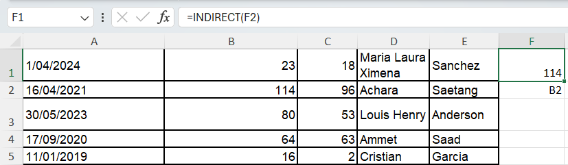
It shows the address of a cell as text.
Examples and variations:
=ADDRESS(3;5)
These formulas are used for financial analysis, testing, and calculations, letting you understand the financial state of a project. Some of the most common formulas are:
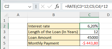
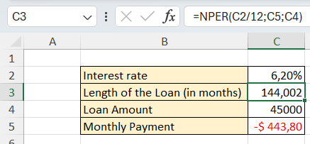
All of these discover certain information about the payment of a loan. PMT calculates the periodic payment, RATE discovers the interest rate, and NPER discovers the number of payments you must make.
Examples and variations:
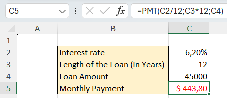
Some of the values must be either multiplied or divided by 12 to make them a monthly value.
It calculates the present value of a loan or investment.
Examples and variations:
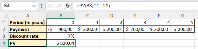
We can see that the example’s present value we would be getting is less than the initial payment we made in period 0. Therefore, this investment is not profitable.
It helps sum up the present values of each cash flow of an investment with variable payment values.
Examples and variations:

According to the NVP, this investment would be profitable.
It discovers the Internal Rate of Return, or the discount rate, at which the NPV is 0.
Examples and variations:

In this case, the IRR is higher than the discount rate. Therefore, this investment is profitable.
It calculates the Future Value of an investment.
Examples and variations:
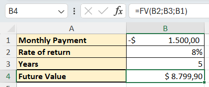
According to the FV formula, we’d get almost $8.800 if we pay $1,500 per each period for five years at a rate of 8%.
These formulas are used for calculating statistical measures. These can be very helpful for analyzing data and understanding your clients. Some of the most common are:
These make an average out of the values that meet specific criteria. AVERAGEIF allows only one condition. While AVERAGEIFS allows more than one criterion.
Examples and variations:
=AVERAGEIF(B1:C5;">30")
=AVERAGEIF(B1:B5;"<50";C1:C5)
=AVERAGEIFS(B1:B5;B1:B5;">50";C1:C5;"<65")
It counts all the cells in a range as long as they’re not empty.
Examples and variations:
=COUNTA(A1:E5)
It counts depending on specific criteria. COUNTIF counts the cells that meet said criteria and works for only one criterion. COUNTIFS counts the times that all the criteria are met in a range.
Examples and variations:
=COUNTIF(F1:F5;"M")
=COUNTIFS(B1:B5;">50";F1:F5;"F")
They sum up the value in cells that meet certain criteria. You can establish more than one criterion with the SUMIFS formula.
Examples and variations:
=SUMIF(F1:F5;"M";C1:C5)
=SUMIFS(C1:C5;F1:F5;"M";B1:B5;">50")
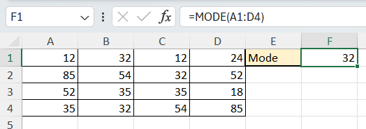
It returns the most frequent value in a range.
Examples and variations:
It calculates the variance through a range of values.
Examples and variations:
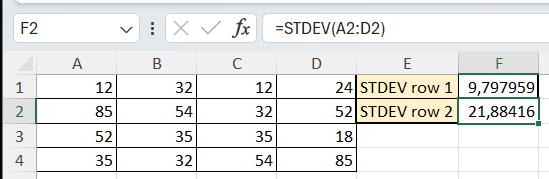
Calculates the Standard Deviation of a range of numbers.
Examples and variations:
Calculates the median of a range of values.
Examples and variations:
=MEDIAN(B1:B5)Returns 64
=MEDIAN(C1:C5)Returns 53
Some formulas help you with more complex dynamics. Some of those formulas are:
It applies a formula to an entire range of cells simultaneously. Allowing you to save time and manage large amounts of data. You use it by writing the operation you need to do and then exiting with Ctrl+shift+enter to make it work.
Examples and variations:

If you see the “{}" in your formula, it means you’re using an ARRAYFORMULA.
It returns a value from a cell or range, relative to another reference cell.
Examples and variations:
=OFFSET(B1;3;1;1;1)
=OFFSET(C2;3;-1;1;1)
As you can imagine, all these formulas open up immense possibilities for Excel usage. Anyone can employ it for various purposes. Mastering Excel formulas will undoubtedly enhance your productivity, whether you're analyzing data or organizing budgets and datasets. The possibilities are truly endless.
It’s important to remember that kill comes with practice, and the more you use these formulas, the better you'll understand how to apply and combine them to maximize effectiveness. The more you delve into them, the more you'll find yourself falling in love with Excel.
For Excel enthusiasts, consider a yearly lookup for updates among the 400+ functions. Otherwise, stay informed about major updates and tailor your research to your specific Excel needs.
Not really. Excel provides information on each function's purpose and tell you what’s the required data for accurate results. Just pay attention to the pop-up information.
Create scenarios and datasets in which you can use the formulas you’re interested in. Look for tutorials around that let you download the spreadsheet they’re using in the video so you can practice.
You can click on the warning sign when an error appears, and it will explain to you what is wrong so you can fix it.
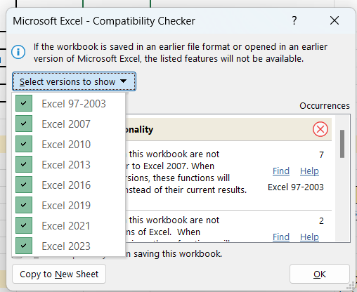
To make sure, you can always use the compatibility checker in Excel.